Notes on Non-adversarial Invariance

There have been a few questions about our Invariant Representations paper from last year's NeurIPS. Since a lot of the questions overlap, and since I think the core idea of the paper is fairly basic once understood, I decided to write a short tutorial to try to explain the intution, and to provide a worked Keras example. The code and a jupyter notebook version of the notes can be found in this github repo, which is written in TF/Keras.

I'm definitely not a blogger (and this is definitely not a blog yet), so go easy! Please let me know if there ways to improve this.

This tutorial requires basic variational auto-encoder knowledge, and some information theory knowledge, but otherwise should hopefully be pretty accessible. If you're not familiar with VAE, there's a great tutorial from Lilian Weng here. I should find a good IT for ML tutorial, but I haven't yet, so if you know of a good one please link me and I will add it here! The standard reference text is Cover and Thomas [amazon link] , but that's complete overkill.

We'll start by building up adversarial invariance (that is, learning invariance using adversarial training), then we'll take a short walk through the math of what invariance is attempting to do more generally. From this we'll construct an adversary-free invariance technique, and then we'll implement it.

THIS IS NOT RELATED TO ADVERSARIAL EXAMPLES. Unfortunately there's a collision in terminology. We're talking about learning statistically invariant features, meaning $p(z|c) = p(z)$, not learning features that can't be changed under some adversarial optimization $opt_x(p(z|x))$. The second set of work is super interesting and completely unrelated as far as I know.

Background: Adversarial Invariance

A surprisingly large amount of Machine Learning literature is about learning to ignore information. Examples include:

classic vision tasks of generating features that ignore scale, or rotation, or shifts,
the statistical task of ignoring/regressing out specific confounders or instrument effects
the more recent task in algorithmic fairness of ignoring information that would bias us against specific protected classes

A lot of work has done this analytically, for specific outside factors (e.g. rotation in images). This works best when we have a good analytic description of the effect.

In more general cases however, analytic solutions are not accessible. This is amplified somewhat by the rising use of neural networks, which themselves are usually not amicable to analytic results. In these cases a common solution is adversarial training, which we''ll now construct informally.

Notations: data $x$, encodings $z$, protected classes $c$, abstract primary task $\mathcal{L}$ for which we want $c$-invariant solutions.

Recipe for adversarial invariance: Train your favorite feature encoder $q(z|x)$, probably a deep network, for task $\mathcal{L}[q(z|x)]$. Train an adversary $a(c|z)$ that tries to predict protected class $c$ from encoding $z$. If the adversary cannot predict $c$, congrats! We're invariant (up to our adversary $a$ and its training). If not, train $q(z|x)$ some more, this time adding the negative accuracy of $a(c|z)$ to $\mathcal{L}$, so that hopefully $q$ will both solve $\mathcal{L}$ and not let the adversary $a$ be predictive of $c$. Retrain the adversary and repeat.

In even more informal language, adversarial training sets up a chump $a$ for $q$ to fight against. Our chump adversary $a$ tries to predict what $q$ is trying to forget, and $q$ in turn tries to hide this information from $a$ while still accomplishing its primary task.

This concept was discovered/introduced in the literature at least three times, albeit for different applications:

Adversarial training is easy (conceptually), works well in many cases, and is fairly flexible in that it can be applied to many diverse situations. In practice I think you should always try the adversarial learning setup.

So then why did we publish a paper about anything else? Our paper isn't trying to rag on adversarial training.

Well, we got curious about the theory behind adversarial invariance. Digging into this theory we found a separate set of results. In my opinion, these derivations provide good intuition for the invariance task in general; they suggest for adversarial cases a specific error mode which can be avoided, and they also suggest a method which approaches the general invariance criterion from the other side (literally, the other side of an inequality), a non-adversarial training scheme.

We started digging into the theory with a more formal rephrasing of the adversarial objective. Again denoting our data as $x$, the encoding as $z$, and the outside variable $c$ (that we want to remove from $z$), the adversarial solution under Cross Entropy loss can be written as this minimax game \[ \Large \min_{q(z|x)}\max_{a(c|z)} ~~ \underbrace{ \mathbb{E}_{x,c}[ \mathbb{E}_{q(z|x)}[ ~ -\log a(c | z) ~ ] ~ ] }_{\text{Adversarial Inv.}} + \underbrace{\mathbb{E}_{x\vphantom{q(z|x)}}[ ~\mathcal{L}[q(z|x)] ~]}_{ \text{Primary Task} } \] Here, the best of all possible adversaries is the "actual likelihood" $p(c|z)$ (this result can be seen from the properties cross-entropy).

This adversarial cross-entropy term can be transformed into mutual information by adding a constant entropy term, and that is where our story really begins: \[ \Large \underbrace{\inf_{a} ~\mathbb{E}_{q(z|x)}[ ~ -\log a(c | z) ~ ] ~ ]}_{\text{Best Case Adversarial Inv.}} ~= -H(c|z)\] \[ \Large H(c) - H(c|z) = I(c,z) \]

Minimal Mutual Information

What we would really like to do is minimize mutual information, either through adversarial methods or otherwise. Invariance is statistically the same as $z \perp c$, and the minimal mutual information condition is a tractable relaxation of this. Once we know this fact, we can attempt to attack the problem directly. Doing a little math, we arrive at the following bound: \[ \Large I(z, c) \leq \underbrace{- \mathbb{E}_{x,c,z\sim q}[ \log p(x|z,c)]}_{\text{Reconstruction}} + \underbrace{\mathbb{E}_{x}[~KL[~q(z|x)~\|~q(z)~]~ ]}_{\text{Compression}} - \underbrace{\vphantom{\mathbb{E}_{x,q}[]}H(x|c)}_{\text{Const}} \] Here, the compression term is a synonym for $I(z,x)$, and in that term $q(z)$ is the empirical marginal: \[ \Large q(z) = \int q(z|x) p(x) dx \] Minimizing this bound is a different proxy for minimizing $I(z,c)$, one that is a) loose in the conservative direction (always an upper bound, while adversaries are always a lower bound), and b) trades adversarial inaccuracy for conditional reconstruction error. In the adversarial set up, our error came from the inaccuracy of the adversary in approximating the best of all adversaries. In this set up, the looseness of our bound is from the inaccuracy of the reconstruction term. Further, if we can do perfect reconstruction, this bound is actually an equality.

There are only two things we can touch in this bound: the encoder $q(z|x)$ and the conditional decoder $p(x|z,c)$. In the next section we'll talk about implementation, but first I think it's important to talk about this intuition: the invariance bound we found is exactly compressive encoding plus conditional reconstruction. This means that if you compress (restrict the channel between $x$ and $z$) and you do conditional reconstruction, you will induce invariance to whatever you conditioned on.

That's it. That's all there is to it. This bound is as tight as the error of the conditional decoder, so if you can auto-encode successfully, and you're using a compressive encoding, you'll get invariance. This is, in my opinion why the Variational Fair Auto-Encoder works so well. It also, in my opinion, illustrates the importance of the Rate-Distortion view of auto-encoders. We derived this without knowing about the distribution $q(z|x)$, so if you choose a different noise model besides the usual conditional gaussian we can still learn invariant representations. In fact, we didn't even assume that $q$ and $p$ are neural networks, so if you have a separate parameterization (GPs?), you could use that and still have exactly the same $I(z,c)$ bound.

If you can't auto-encode, or if auto-encoding/reconstruction is expensive, you should use one of the adversarial methods. Remember, they're still okay! Give your adversary more training epochs, maybe even different training dynamics, and it hopefully will work out.

Implementation for Gaussian VAE

The "TODO List":

Make a Gaussian encoder, $q(z|x)$.
Make a conditional decoder, $p(x|z,c)$.
Implement the compression: $I(x,z) = KL[~q(z|x)~\|~q(z)~]$

Here's a picture of where we're going:

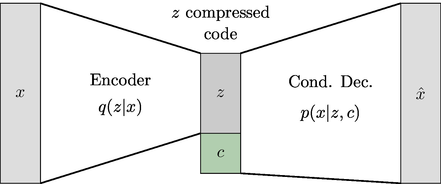
If we choose to do this for conditional gaussian $q(z|x)$, our implementation will look a lot like vanilla conditional VAE. Encoder and decoder are almost straight out of the Keras Tutorial, with an additional $c$ input at the latent rep. layer $z$.


#declare inputs to the encoder, which is just x
input_x = keras.layers.Input( shape = [INPUT_SHAPE], name="x" )

enc_hidden_1 = keras.layers.Dense(512, activation=ACTIVATION, name="enc_h1")(input_x)
enc_hidden_2 = keras.layers.Dense(512, activation=ACTIVATION, name="enc_h2")(enc_hidden_1)

#first output, z_mean
z_mean = keras.layers.Dense(DIM_Z, activation=ACTIVATION)(enc_hidden_2)
#second hidden output, z_log_sigma_sq.
z_log_sigma_sq = keras.layers.Dense(DIM_Z, activation="linear")(enc_hidden_2)

#stolen straight from the docs
#https://keras.io/examples/variational_autoencoder/
def sampling(args):
    z_mean, z_log_var = args
    batch = K.shape(z_mean)[0]
    dim = K.int_shape(z_mean)[1]
    return z_mean + K.exp(0.5 * z_log_var) * K.random_normal(shape=(batch, dim))

z_mean = keras.layers.Dense(DIM_Z, activation="tanh")(enc_hidden_2)
z_log_sigma_sq = keras.layers.Dense(DIM_Z, activation="linear")(enc_hidden_2)

z = keras.layers.Lambda(sampling, output_shape=(DIM_Z,), name='z')([z_mean, z_log_sigma_sq])

#declare any additional inputs to our decoder, in this case c
input_c = keras.layers.Input( shape = [DIM_C], name="c")
#this is the concat operation!
z_with_c = keras.layers.concatenate([z,input_c])

dec_hidden_1 = keras.layers.Dense(512, activation=ACTIVATION, name="dec_h1")(z_with_c)
dec_hidden_2 = keras.layers.Dense(512, activation=ACTIVATION, name="dec_h2")(dec_hidden_1)

x_hat = keras.layers.Dense( INPUT_SHAPE, name="x_hat", activation="linear" )(dec_hidden_2)

So far we've got a path from $x$ to $z$ and then from $(z,c)$ back to $x$. Note that this is just one way to implement the conditional dependence of $p(x|z,c)$, and a particularly weak and naive one at that. There isn't to my knowledge a standard way of doing this yet. In this one, we just concatenated $z$ and $c$. Fader networks suggested concatentating at every output layer. There are probably even better ways of doing this, and if you know about them I would love to know about them too, email me and we can list them here.

Okay, let's build the loss functions. There are three terms:

Reconstruction $\|x - \hat{x}\|$
Shrinkage to Prior $KL[ ~ q(z|x) ~ | ~ \mathcal{N}(0,I) ~ ]$
Shrinkage to Posterior $I(x,z) = KL[~q(z|x)~\|~q(z)~]$

The reconstruction loss is built into Keras, and the prior loss is pretty easy to construct for diagonal gaussians (see the Wikipedia page). The third loss we will approximate using per batch all-pairs KL divergence. The tensor form of this is a bit involved, but the code is on the github. It is quadratic in batch-size, and only contains linear and elementwise operations.


params = {
  "beta" : 0.1,
  "lambda" : 1.0,
}

recon_loss = keras.losses.mse(input_x, x_hat)
recon_loss *= INPUT_SHAPE #optional, in the tutorial code though

prior_loss = 1 + z_log_sigma_sq - K.square(z_mean) - K.exp(z_log_sigma_sq)
prior_loss = K.sum(prior_loss, axis=-1)
prior_loss *= -0.5

#see src/kl_tools.py
kl_qzx_qz_loss = kl_tools.kl_conditional_and_marg(z_mean, z_log_sigma_sq, DIM_Z)

#full loss
icvae_loss = K.mean(
  (1 + params["lambda"]) * recon_loss + 
  params["beta"]*prior_loss + 
  params["lambda"]*kl_qzx_qz_loss
)

Okay! So now we have a network and we have losses. We can choose a dataset, compile it all together, and train it.


icvae = keras.models.Model(inputs=[input_x,input_c], outputs=x_hat, name="ICVAE")

icvae.add_loss(icvae_loss)

learning_rate = 0.0005
opt = keras.optimizers.Adam(lr=learning_rate)

icvae.compile( optimizer=opt, )
icvae.fit(
    { "x" : train_x, "c" : train_y }, epochs=100
)

Some MNIST Results

This section uses the vanilla MNIST dataset with


#these variables were actually defined BEFORE the previous sections
DIM_Z = 16
DIM_C = NUM_LABELS # just as an example. Sometimes we also have another y
INPUT_SHAPE = IMG_DIM ** 2
ACTIVATION = "tanh"

As a first check, we can look at the reconstruction. These are straight out of the notebook, so my apologies for quality.

Even with minimal tuning and/or extra stuff, it seems to do fairly well. This is because the conditional auto-encoding task is MUCH easier than the non-conditional version. The outputs are fuzzy, but we can try to get rid of this by using a more powerful decoder, an image measure that isn't L2, and by using the mean embedding. And probably a billion other tricks.

Okay, now for the more fun manipulation test: changing $c$ at test time. From left to right we have the original, then the reconstruction, then the reconstruction with $c=0,\dots,9$.

Okay, so while it doesn't work amazingly well (...some of those 2s and 9s are questionable), it is doing two things correctly:

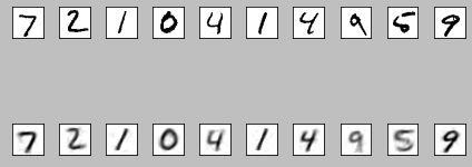
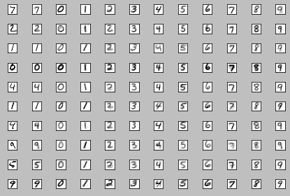
Removing the input digit class, e.g. we can't see residual 0 bits when mapping 0 to other digits.
Transfering some elements of the style, notably how dark digits are, how tilted each digit is, and their approximate vertical alignment.

Wrapping up Part 1

So we just constructed in theory and in 20ish lines of TF/Keras an invariant VAE. In my opinion, this exercise wasn't about building a SOTA invariance method, nor was it to say that adversaries are universally bad. It was, for me, more to link adversaries to $I(z,c)$, and then link $I(z,c)$ to compression. We can come at $I(z,c)$ from both directions now, with upper and lower bounds, and we related it to an existing task, compressive reconstruction.

Again, everything here can be found in this github repo.

Next up next week(?): more theory for alternate $I(z,c)$ regularization, and an invariant prediction method.